
Technology · Piesis
One synthetic section, worked through.
Piesis is a steady-state circulating hydraulics engine: annular pressure and ECD from surface to TD, and standpipe pressure leg by leg, for conventional and managed-pressure wells.
Most hydraulics questions on a narrow-margin section are steady-state questions, and they tend to be answered either in a full transient simulator or in a spreadsheet that shows its answer but not its assumptions.
The annulus is marched from surface to TD on published, cited correlations, and the solved case is read against the pore and fracture curves.
Screenshots use synthetic or published data. No client record, well, result or proprietary method appears in any image on this page.
Every screen below is the application’s own built-in example — an invented, deviated 8½-in managed-pressure section — at its default settings. The numbers in the images belong to that example and to nothing else.
Walkthrough
From the survey to the operating window.
- 01
The well, from its survey
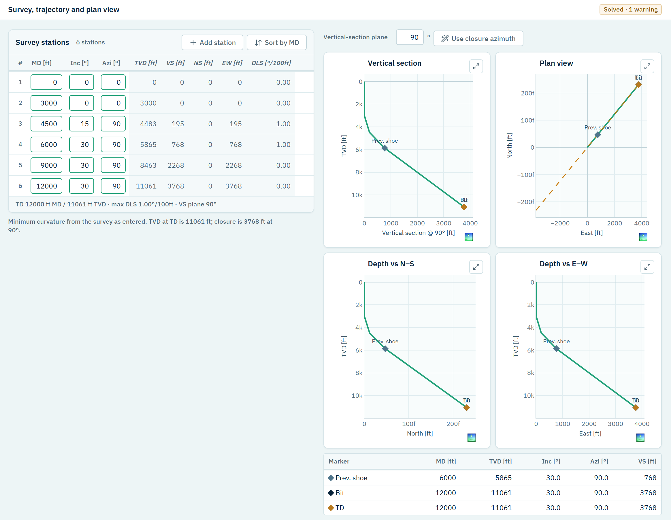
Six survey stations become TVD, vertical section and plan view by minimum curvature, with dog-leg severity alongside each station.
This is checked before any hydraulics is believed: a spike in dog-leg severity, or a step in inclination, is almost always a mistyped station — and every pressure below would inherit it.
- 02
The annulus it will be solved through
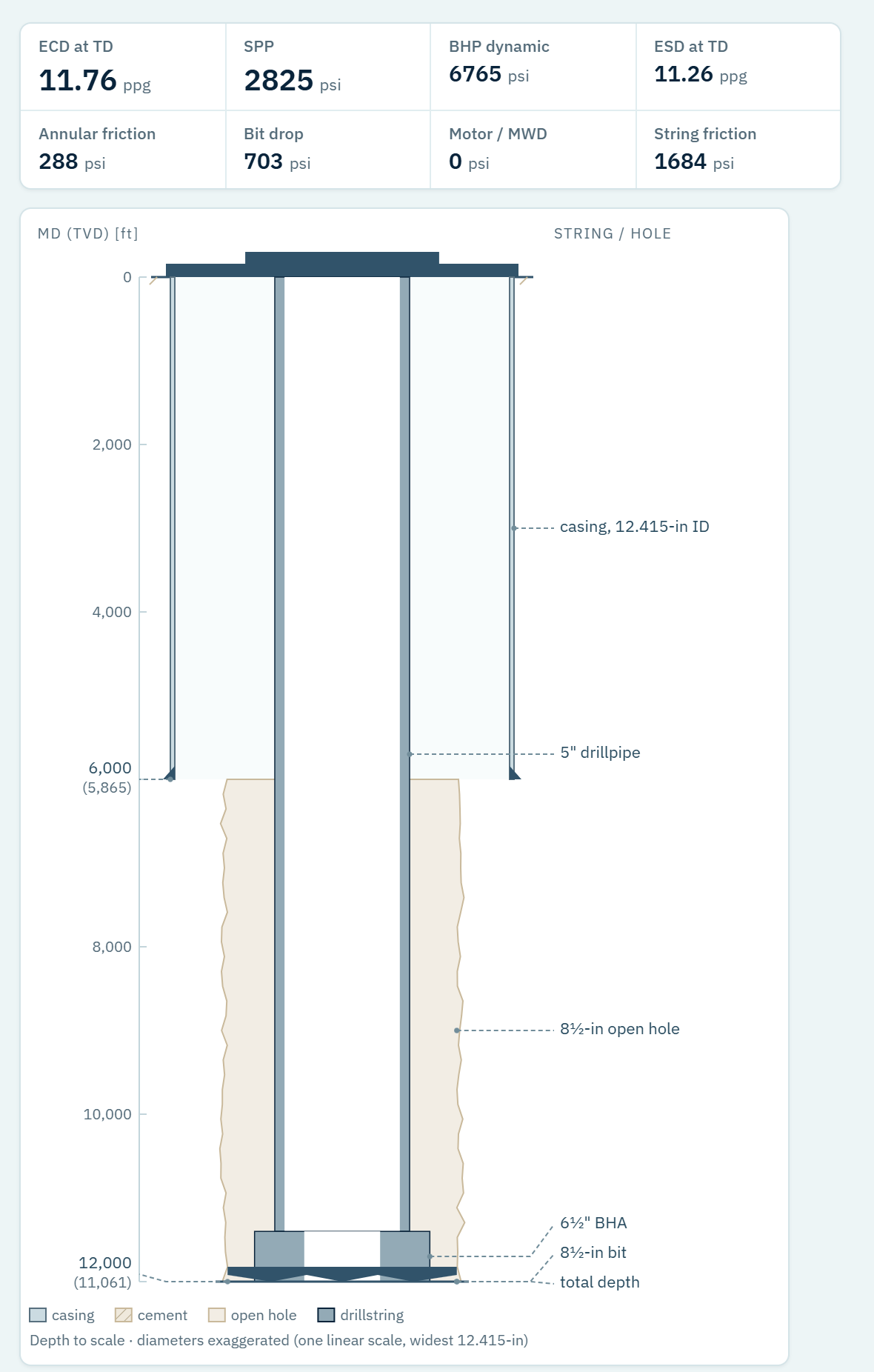
Casing to the shoe, open hole below it, drillpipe and BHA, drawn with depth to scale and diameters exaggerated on one linear scale.
The geometry is seen before it is solved, so a diameter entered in the wrong row is caught by eye rather than discovered later as an annular friction nobody can explain.
- 03
The mud, as it was measured
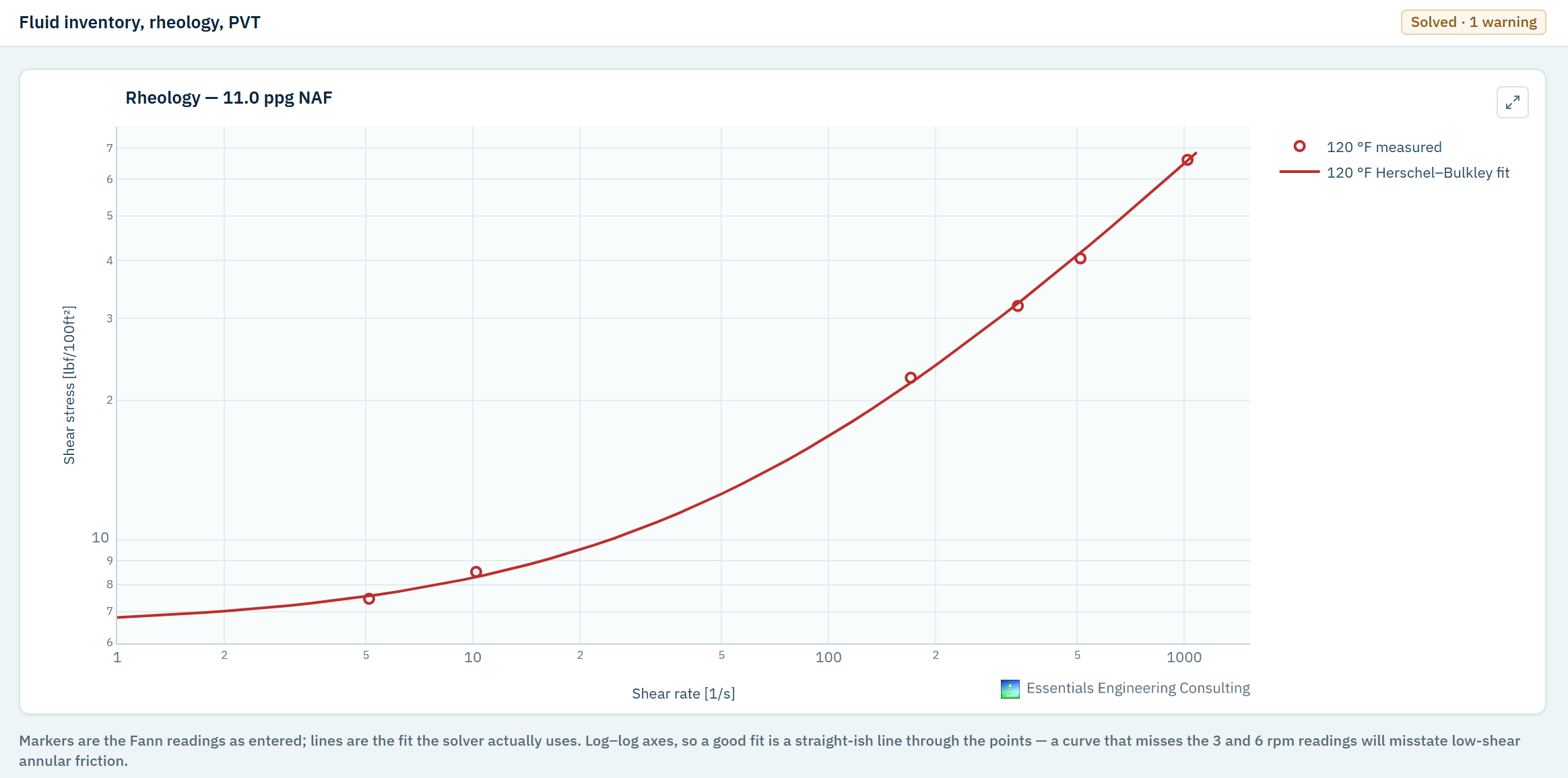
Viscometer readings are entered as read, and the Herschel–Bulkley fit the solver actually uses is drawn through them on log–log axes.
The fit is judged against the points, not accepted as three parameters: a curve that misses the 3 and 6 rpm readings will misstate low-shear annular friction.
- 04
Standpipe pressure, leg by leg
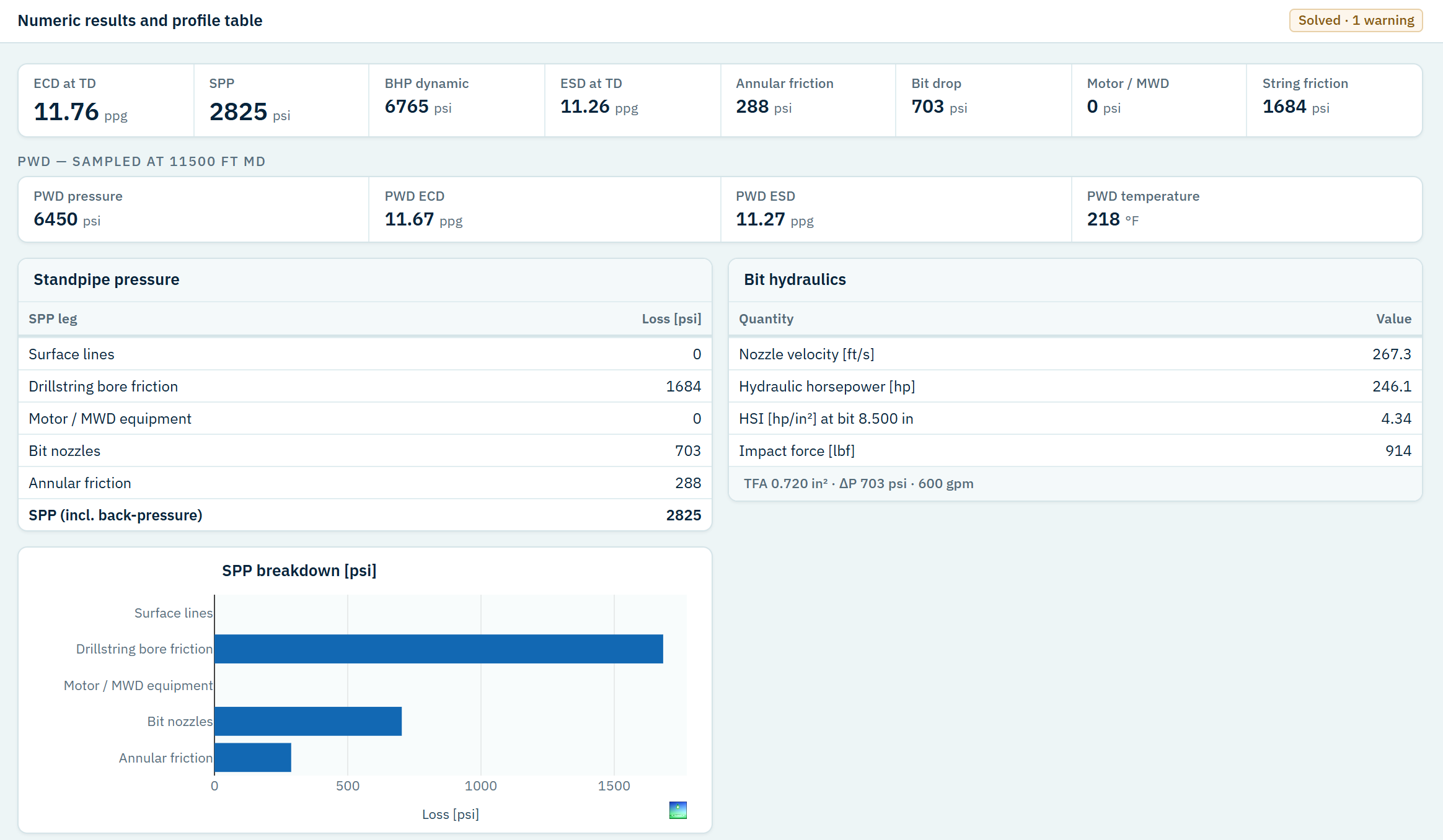
ECD, standpipe pressure and bottomhole pressure at the current rate, with the standpipe pressure assembled from surface lines, string bore, motor and MWD, bit nozzles and annulus, and the bit hydraulics beside it.
Two legs read zero on this case, and they stay in the breakdown. A measured standpipe pressure that disagrees with the total can be traced to a leg, rather than argued with as one number.
- 05
The rate window, and what binds it
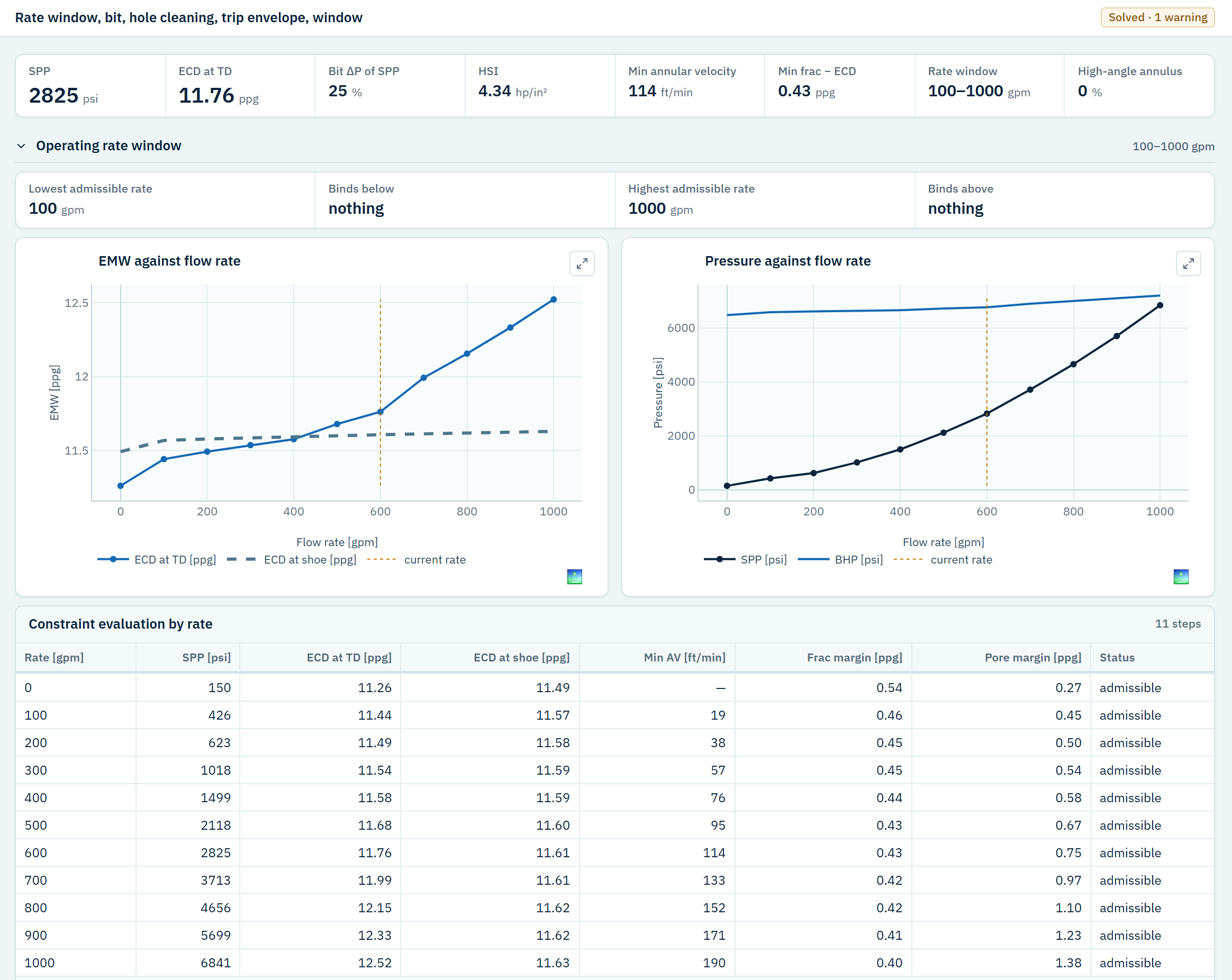
Every rate in the sweep is solved in full and checked against the pore and fracture margins: ECD at TD and at the shoe, standpipe and bottomhole pressure against rate, and the evaluation rate by rate.
Here nothing binds the window at either end, and the screen says so in as many words — the case carries no operating limits, and the engine supplies none of its own.
- 06
The operating window, drilled from shoe to TD
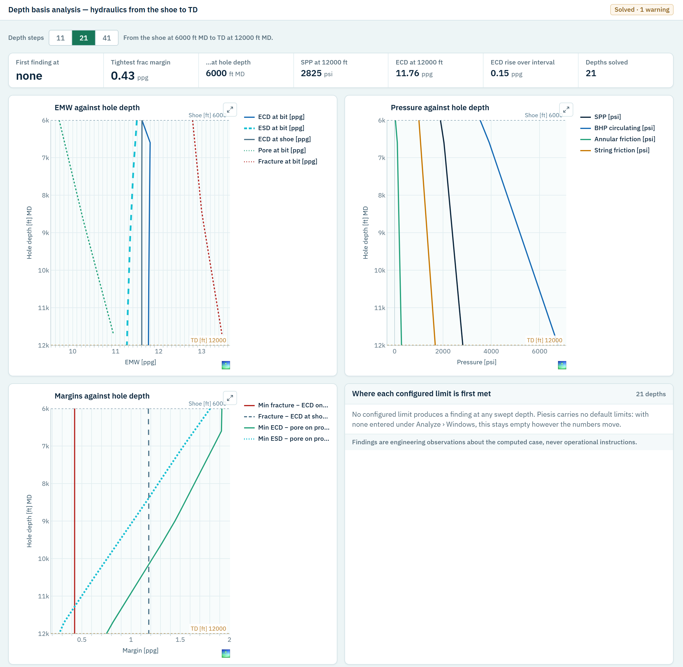
The section is drilled step by step from the shoe to TD, with a full solve at every hole depth, and read against the pore and fracture curves: ECD and ESD at the bit, the pressures, and the margins on both sides.
It answers where in the section the window gets tight — a depth, not a single number — and lists where each configured limit is first met.
A hydraulics question of your own?